Ring Attention: Shedding Light on the Dark Art of Attention Sharding

Healthcare documentation demands models that can process long-context medical documents and massive sequences. But standard attention mechanisms break down long before reaching that scale.

Overcoming this requires rethinking how activations are stored and shared across devices. This post explores how we used Ring Attention to scale large language models (LLMs) into the 100k+ token regime.

First introduced by Liu et al., Ring Attention is a distributed extension of Flash Attention, which allows scaling maximum context windows by simply increasing the number of GPUs.

We will outline the detailed step-by-step process of how a popular LLM was scaled from just tens of thousands of tokens to hundreds of thousands of tokens using parallelism across only four GPUs, providing thorough profiling analysis to motivate each step, and illustrating several subtleties that arise when putting this algorithm into practice.

Background: Baseline Memory Requirement for Training

Throughout this post, we will focus primarily on the compute and memory dynamics for finetuning Llama 8B. The optimizations outlined can be readily extended — without loss of generality — to a model of any parameter size, as long as the underlying GPU specifications allow for these improvements. Supervised finetuning for Llama 8B exhibits the following memory profile over two training steps on a single H100 GPU (80 GB of VRAM).

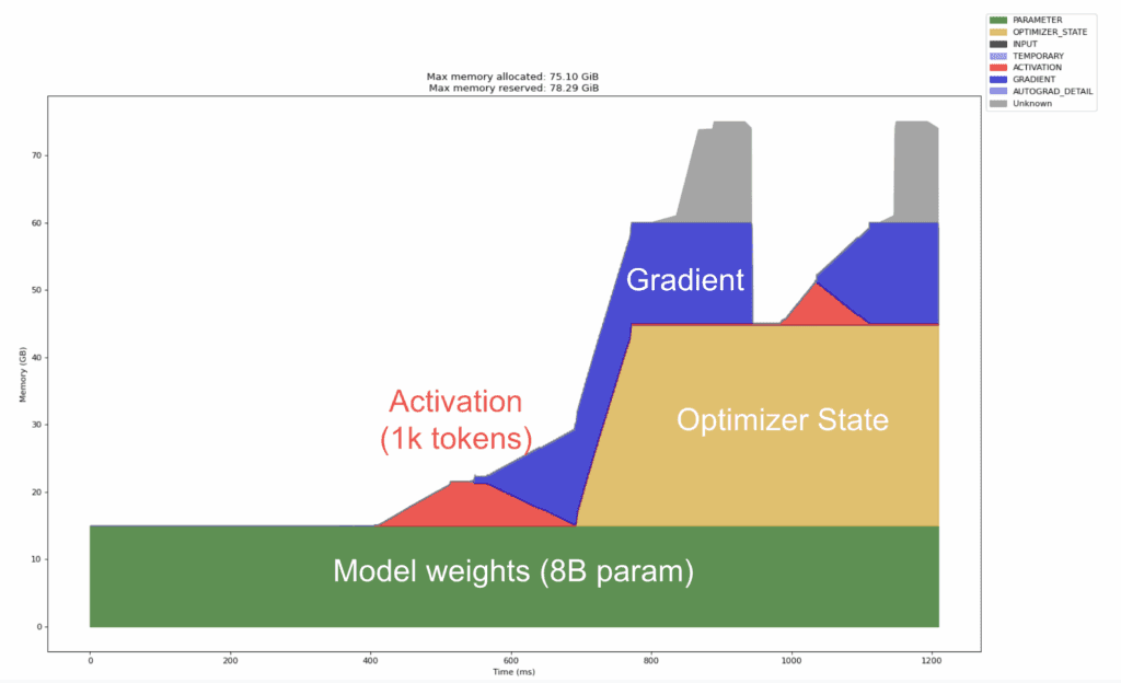
Figure 1: Baseline memory requirements for Llama 3.1 8B model.
(The diagram is generated in a similar manner as in the PyTorch blog.)

All necessary training components are fully materialized on a single GPU. The context window is constrained to 1000 tokens to remain within the 80GB limit. Looking at the diagram above, the four components that dominate GPU RAM are:

• Model weights (green block): The tensors that define the network itself. Memory scales linearly with the number of parameters, P. For the 8B model, it will take up ~16GB in GPU memory in bf16. They are persistent in GPU memory throughout training.
• Gradients (blue block): The gradients of the loss with respect to the model parameters. Memory scales linearly with the number of parameters P, and it is another ~16GB in GPU memory.
• Optimizer state (tan block): Common optimizers, including Adam/AdamW, maintain first and second moments for every parameter. They are moving averages of the gradients. The first moment acts like velocity; it carries updates forward in directions that have been consistently good, creating a momentum for updating model weights. The second moment tracks how bumpy each weight’s gradient is and scales steps down on noisy/steep parts, so the momentum stays smooth instead of jittery. These two add approximately 2× model‑size memory requirements. For the 8B model, it will take up an additional ~32GB in GPU memory, as each moment can be represented with bfloat16s. The optimizer state is fully allocated in GPU memory when the backward pass is first called.
• Activation: Intermediate outputs retained for backward computation. Unlike the above, usage is driven primarily by sequence length n and model depth; for attention, growth is O(n2) and will become the dominant factor as the context window increases.

Common Training Optimization

A single 80 GB H100 is already saturated at ~1k tokens, so practical long‑context finetuning requires distributing the training state across multiple GPUs — starting with model sharding.

By applying parameter sharding (e.g., FSDP FULLY_SHARD) across four devices, each GPU holds only a quarter of the model weights, optimizer state, and gradients. This immediately reduces per-device memory for these components, freeing up headroom for larger batch sizes or longer context windows.

We can monitor and visualize the active GPU memory usage within a single GPU with the PyTorch Profiler. Below is an example profiler output of the aforementioned setup with FSDP fully sharding the Llama 3.1 8B model across the four devices, with sequence length at 1000. Each device shares a similar memory profile, so only the graph of one of the devices is shown for brevity. Unless otherwise mentioned, training batch size is kept to 1 for all runs, and Flash Attention 2 is enabled by default.

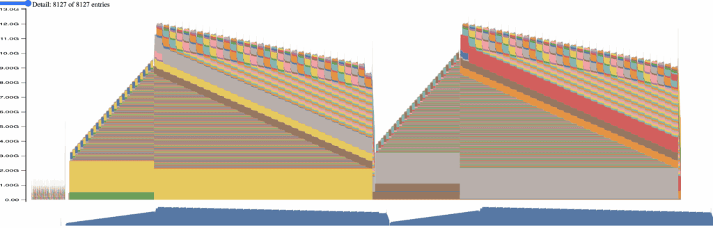
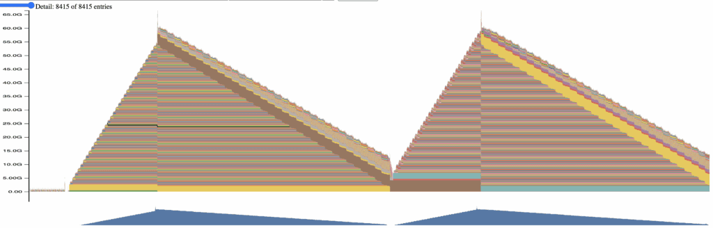
Figure 2: Memory footprint of fully sharding at 1k tokens
(These memory profile figures are collected using the built-in PyTorch Profiler feature and visualized through the official documentation site. Note that the profiler is enabled after the model weights are initialized and split across devices. This can cause the profiler to lose track of some of the model parameters.)

The profiler records every memory allocation and deallocation event, so it can be noisy. Below is a simplified view where the major components are visualized across a single forward and backward pass.

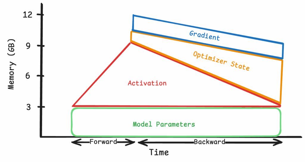
Figure 3: Simplified view of fully sharding at 1k tokens

Model weights, optimizer states, and gradients are sharded across four devices, occupying much less space within a single GPU and reducing the peak memory footprint to just below 12GB, a sizable decrease from the 70GB in Figure 1.

With the peak memory footprint just being shy of 12GB, we can substantially increase the context window to 8000 tokens.

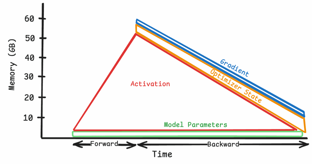
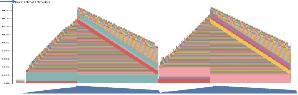
Figure 4: Simplified view of fully sharding at 8k tokens
(refer to Appendix 2 for the memory profiler blueprint)

As sequence length grows, activations, not parameters, become the dominant bottleneck. Flash Attention 2 and Gradient Checkpointing are common approaches to alleviate this bottleneck, but they don’t resolve it as the sequence size grows past a certain value.

Furthermore, Flash Attention uses on-device block-based attention computation to bring down the memory complexity of attention to O(n), albeit with a very large constant which grows with sequence length. (Refer to Table 1 in Ring Attention Paper.) Gradient checkpointing can also reduce the peak activation memory by recomputing intermediates (we will go into more details in the later section), but it still requires all activations to be computed on the same device. To truly scale, we must treat activations like parameters and distribute them across multiple devices.

Ring Attention does exactly this: it splits the attention activation across GPUs so each device holds only a fraction of the sequence while computing the same result.

Ring Attention

The idea of breaking up the attention matrix into smaller chunks and computing them in a block-wise manner is not new. It is introduced in the Flash Attention paper as a way to reduce the memory footprint of the attention computation and improve training efficiency by sizing each chunk to the high-speed but small high-bandwidth memory (HBM) of the GPU.

The very idea of blockwise attention is explained in its own paper: Blockwise Parallel Transformer for Large Context Models. Ring attention leverages a similar idea and focuses on partitioning the attention block to fit within the GPU’s total memory.

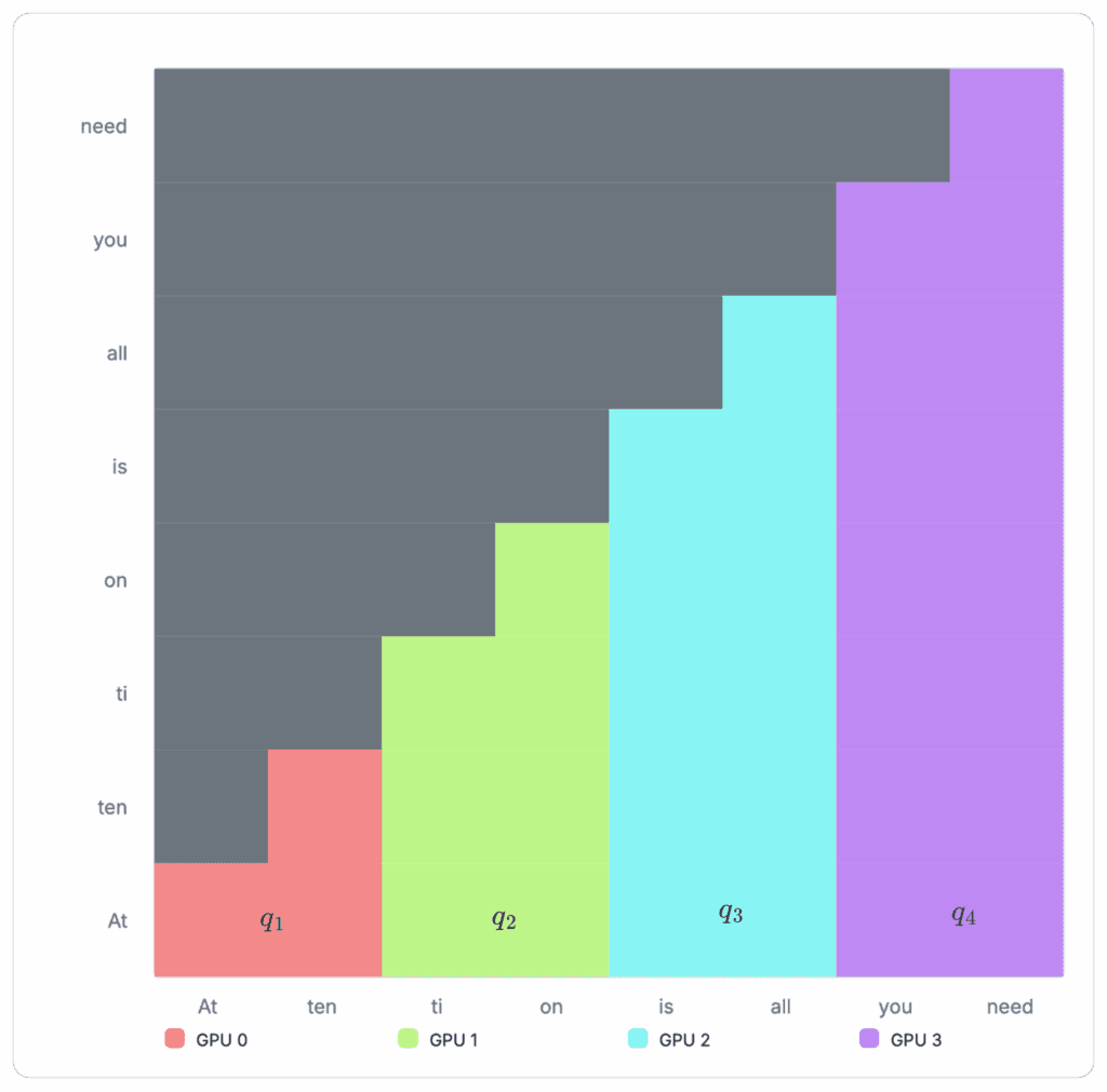
Suppose we have the following sequence of tokens: “Attention is all you need”. We can visualize the attention matrix for this sequence as follows:

Figure 5: Example attention matrix

Each red block is a score indicating how much the specific token should attend to itself and other tokens in the sequence. For causal attention, tokens will only need to attend those that come before it. Attention will not be computed for later tokens. This masking behavior is visualized as the gray blocks in the diagram, resulting in a signature triangular stair-stepping shape.

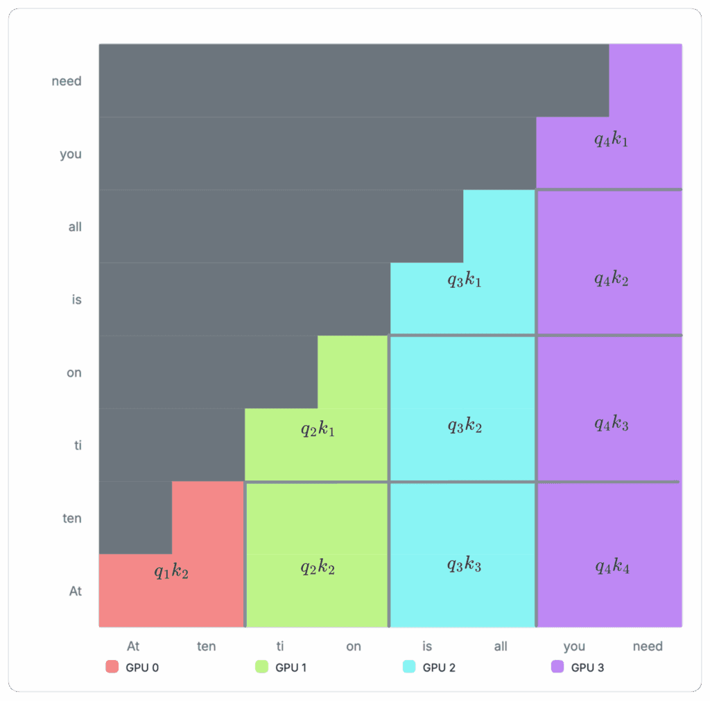
Figure 6: Example cross-device allocation with Ring Attention

Ring attention can segment the above matrix into separate GPUs, so each GPU only needs to compute its own share. The example sequence is now split into four separate chunks and assigned to four devices: GPU 0 receives two tokens, “At ten”. GPU 1 receives “ti, on”, GPU 2 receives “is all,” and GPU 3 receives “you need”.

To compute the assigned section of the attention matrix, each GPU first computes the attention block currently stored in its memory, then passes the results to the next GPU that depends on it to compute the next block.

From then, each GPU processes the current block and passes it to the next GPU, while receiving the next block from the previous GPU in a relay-style. This reduction action, which we can refer to as segment parallel, is repeated until the entire attention matrix is computed, as shown in the animation below:

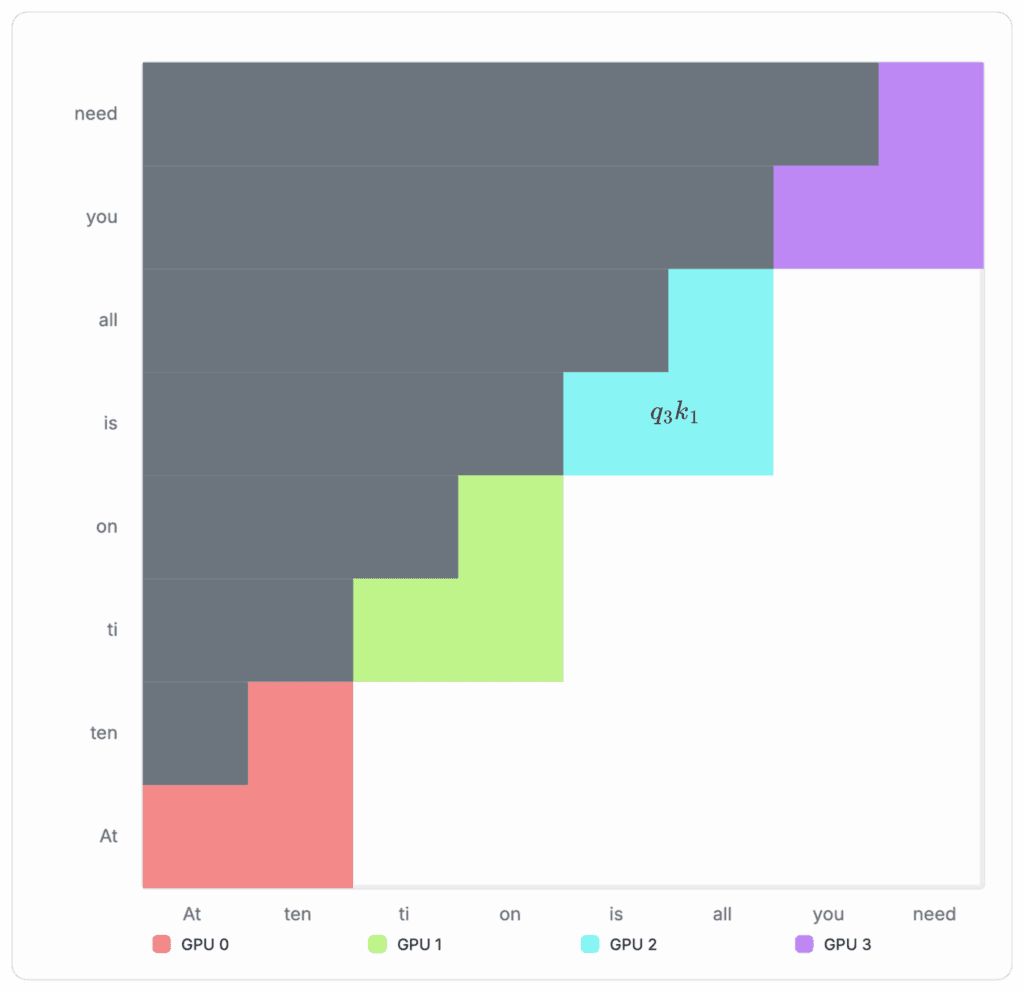
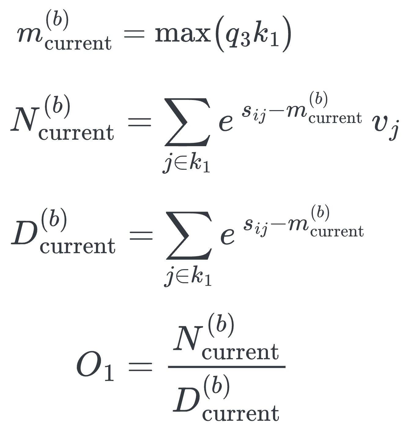
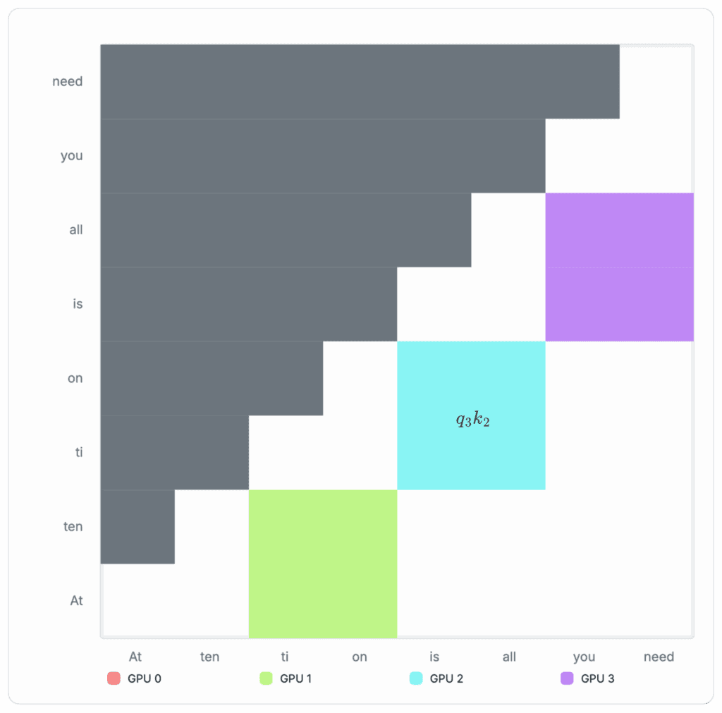
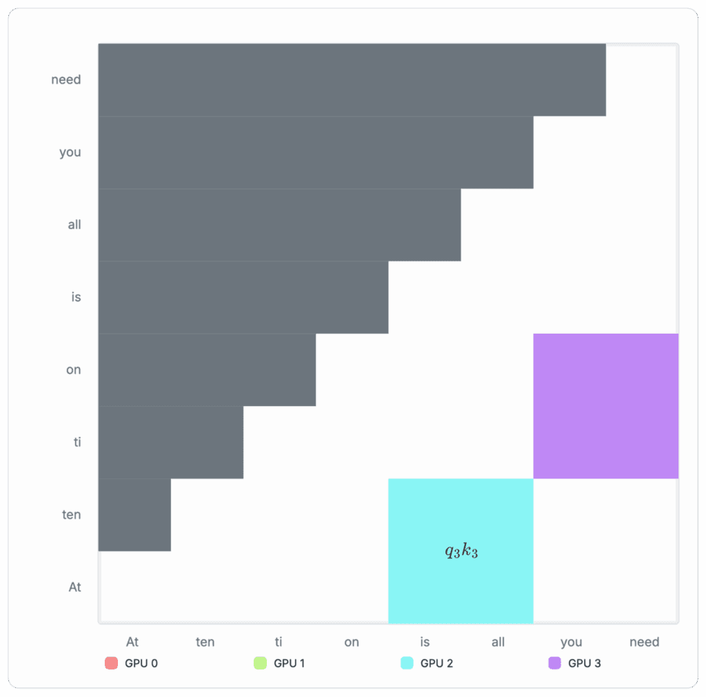
Figure 7: Cross-device computation for Ring Attention

In practice, block-wise attention computation additionally requires storing the accumulated global maximum of the attention matrix for the softmax operation. This is just a constant memory overhead. See Appendix 6 for more details on how this block-wise computation is materialized.

However, Ring Attention is not without trade‑offs. Because each successive segment attends to a larger prefix, computation grows with segment index. Consequently, the later ranks in the ring carry a heavier workload, while the earliest ranks become idle after finishing their shorter initial segments. This is evident in the animation above. Variants such as Striped Attention aim to rebalance this load, but we will not explore them here.

Implementing Ring Attention

Back to optimizing the memory footprint of fine-tuning: With our baseline implementation using FSDP, the GPUs are already almost saturated at 8k tokens. We can now apply ring attention to scale to longer context.

Fortunately, there are existing ring attention implementations we can leverage, such as the one from the author in JAX or from zhuzilin, leveraging the Flash Attention implementation. We will use the latter, as it is more flexible and easier to integrate with the existing PyTorch codebase.

To integrate the ring attention implementation into our fine-tuning pipelines, we made the following changes:

1. Introduced a 2D grid of process groups to separate sequence sharding from data replication

2. Padded the input sequence length to be divisible by the ring size and split tokens into equal and contiguous segments per GPU

2D Process Group Topology

In the baseline distributed setup, we shard model weights, optimizer state, and gradients across four devices (e.g., FSDP) and run four data-parallel replicas for throughput. When Ring Attention is enabled, a single long sequence is split across those same four devices.

To enable data parallelism and faster training, we will use a FSDP_HYBRID_SHARD setting with a two-dimensional process group mesh (replicate, shard):

Figure 8: Example device grouping layout within a node

• Replicate dimension: Standard data parallel replicas that train on independent examples. Each data parallels hold a separate copy of the model and input batch.
• Shard dimension: Ring attention group that partitions both the sequence and model weights across GPUs

This yields world_size = num_replicas × ring_size. Each ring contains ring_size ranks that communicate in a ring during attention. Data parallel replicas never exchange activations with one another. This separation preserves throughput scaling while enabling long-context attention within each ring. For a single node with 8 GPUs, we can have two data parallel replicas and four devices for model sharding and sequence sharding. This setup can be replicated over multiple nodes of GPUs to scale up training.

Sequence Segmentation and Padding

Ring attention requires that each GPU receive a contiguous slice of the sequence. To ensure even partitioning, we pad the effective sequence length seq_len to the nearest multiple of ring_size so we can split the sequence equally into ring_size many sequences. Each individual segment will be allocated to the corresponding ring rank, as depicted in Figure 8.

Note that it is important to assign the segment to the ring rank in a way that maintains the autoregressive ordering. The implementation assumes that ring rank 0 will receive the first sequence segment, ring rank 1 will receive the second segment, and so on.

Profiling Memory Usage With Ring Attention

Using the 2D process group mesh we discussed above, we can enable ring attention across four GPUs with the same sequence length.

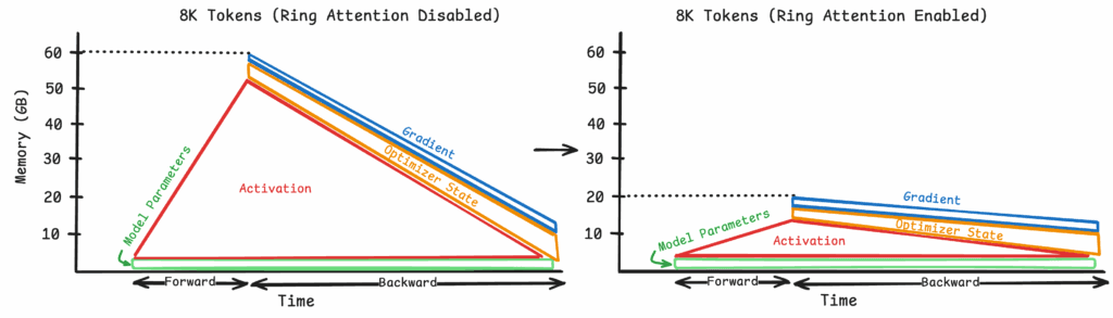
Figure 9: Reduction in peak memory usage with Ring Attention
(Refer to Appendix 2 and Appendix 3 for the corresponding profiler blueprints)

When ring attention is enabled, the peak memory usage is reduced to about 20GB per device from 60GB per device.

In fact, we can further reduce the peak memory usage by enabling gradient checkpointing, a technique that recomputes the activations during the backward pass to reduce peak memory usage.

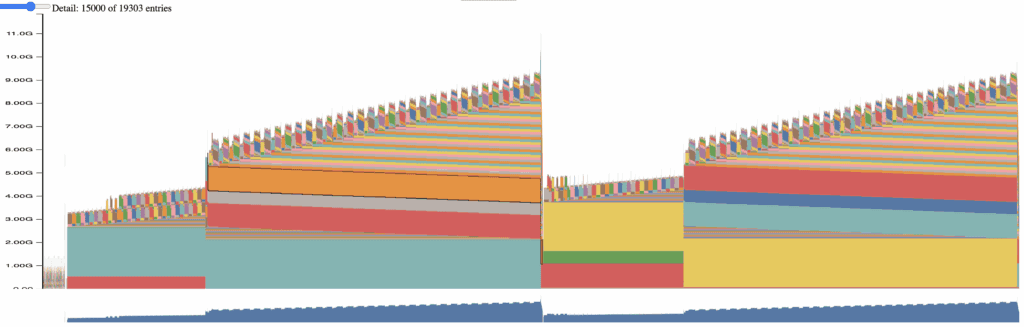
Figure 10: Memory footprint at 8k tokens with all optimizations applied

Figure 10 shows the combined effect of applying the following optimizations across four devices:

1. Model and optimizer sharded via FSDP
2. Ring attention
3. Gradient checkpointing

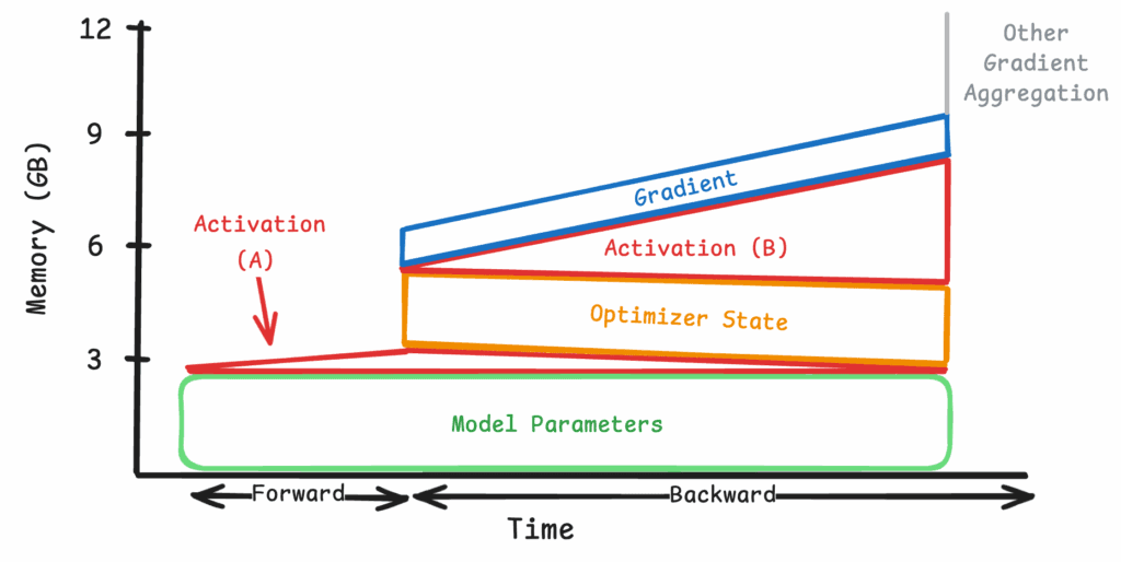
Figure 11: Simplified view of applying all optimizations at 8K tokens

The peak memory usage with 8000 tokens is further reduced to just 12GB per device. Note that the shape of the memory footprint appears very different with gradient checkpointing turned on. Looking at the simplified view in Figure 11, the activation memory usage is now split across two time frames. Its footprint is significantly reduced during the initial forward pass, where only the intermediate model layers are saved (Section A). These unsaved activations are re-computed and materialized onto GPU memory when the corresponding gradients are computed in the backward pass (Section B). In other words, the gradient checkpointing shaves the height of the activation triangle and distributes the memory cost throughout the backward pass.

Combining all of the optimizations together — including model and optimizer state sharding — enabling ring attention and gradient checkpointing, we can scale the training context window to over 100k tokens without maxing out our GPU memory.

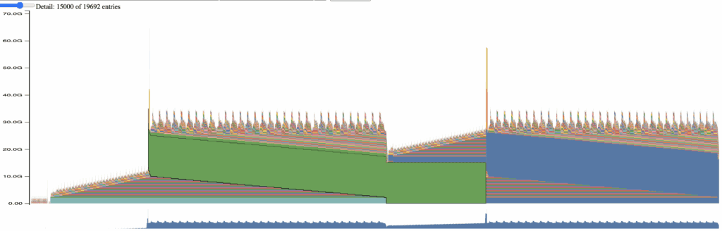
Figure 12: Memory footprint of applying all optimizations at 118K tokens

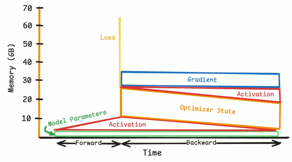
Figure 13: Simplified view of applying all optimizations at 118K tokens

As can be seen in Figure 13, in practice, one is faced with a new bottleneck.

Typically, when calculating overall loss, we observe large spikes in memory usage. This is due to the fact that most loss functions are forced to aggregate activations in the final layer to compute their final values. When computing memory usage statistics, it is therefore important to consider what the peak memory activation is, as this is what causes OOM errors in practice.

In line with this observation, Figure 13 illustrates the peak memory usage during a single training iteration — with and without Ring Attention enabled. All other relevant optimizations, FSDP, and gradient checkpoints are enabled in both setups. This graph clearly shows how ring attention can unlock very long context training while keeping peak memory usage low.

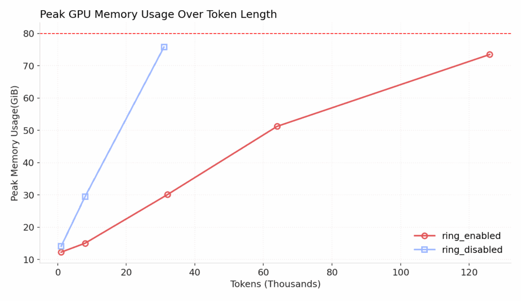
Figure 14: Empirical peak memory usage over different token lengths

In practice, we observe a similar 58% reduction in training throughput as noted in the implementation, due to the increased volume of inter-GPU communication. Overall, this is a small price to pay for the large gains in memory efficiency.

It is also worth noting that we can make up for slower step iteration by increasing the data parallelism across multiple nodes.

Conclusion

We have explored different techniques to optimize model parameters, optimizer states, gradients, and activations, showing how these optimizations enable training large language models like Llama 3.1 8B on sequences ranging from 1,000 to over 100,000 tokens.

These training techniques address a fundamental challenge: The large memory footprint required by each component far exceeds what any single GPU can handle.

By distributing the workload across multiple GPUs, we can leverage collective memory to make training feasible. Ring attention, in particular, enables sequence parallelism that can distribute activations across devices without theoretical limits.

While we demonstrated this approach using four GPUs, the setup scales to any number of available devices. This does introduce computational overhead from inter-GPU and inter-node communication, but, in practice, this trade-off is well worth maintaining the ability to train these large models effectively.

The goal of medical coding is to present the most accurate and comprehensive picture of any medical encounter for the combined benefit of the patient, provider, and payer.

With many complex encounters regularly exceeding hundreds of thousands of words/tokens, it is of great interest to us at AKASA to build LLMs that can attend to every detail of such encounters. Ring attention is, therefore, a vital part of our toolkit for developing systems that bring us closer to this goal.

Appendix

Below are all the footprints we recorded via PyTorch Profiler. They are the blueprints to each simplified view we showed in the content.

Appendix 1: Memory footprint of full sharding at 1k tokens
(Duplicate of Figure 2)

Appendix 2: Memory footprint of full sharding at 8k tokens

Appendix 3: Memory footprint of full sharding at 8k tokens with ring attention

Appendix 4: Memory footprint at 8k tokens with all optimizations applied
(Duplicate of Figure 10)

Appendix 5: Memory footprint of applying all optimizations at 118k tokens
(Duplicate of Figure 12)

Appendix 6: Derivation of Block-wise Attention Computation

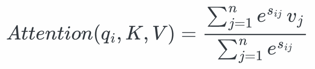
The full attention matrix can be decomposed into a concatenation of the individual Q-columns. Therefore, we can break down the overall attention computation into those associated with the individual Q-columns. To calculate the attention associated with each Q-column, we can sum over:

To calculate the individual Q column (outer for-loop in the block-wise attention algorithm — See Algorithm 1), we can sum over the individual query-key blocks:



Where each σ_ij is the softmax of the corresponding block s_ij, and d_k is the number of features k^th attention head.

This can be further condensed into the following:

To maintain numerical stability, the row-wise maximum logit m_i is subtracted from all logits before applying softmax:

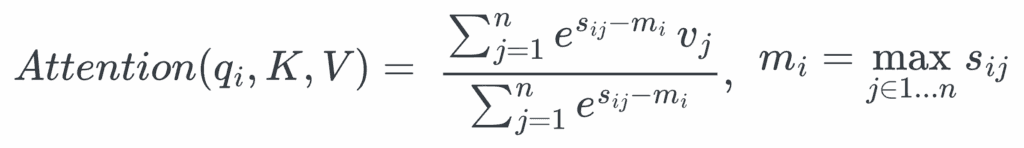
We can further decompose the equation using the relationship between the row-wise maximum m_i and the local block-wise maximum m_i^(b).


To further simplify, this can be viewed as some numerator N_ij over denominator D_ij and both scaled by a common factor α_i.


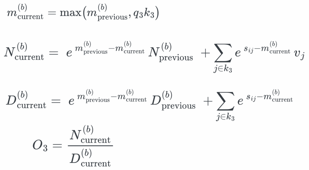
However, during runtime, the global row-wise maximum is not known upfront. We can instead maintain a running max per row as a substitute for the global maximum and renormalize the partial log-sum-exp accumulators whenever a later block raises the maximum:

In practice, this means we only need to remember three running scalars to calculate each Q-column: Running max per row m_i^(b), the running numerator N_i^(b), and running denominator D_i^(b). This is illustrated in the author’s blockwise-attention implementation (see Figure 3).

The process of computing the final attention per Q-column with these intermediate scalars can be visualized in the following diagrams: